
Limits are defined as follows: As an x-value approaches an argument, the two sides of the curve approach the same number. The example above shows the limit as the x-value approaches zero, the two sides of the curve approach zero. When taking the limit of a continuous function (such as x^2), the limit will be equal to the function value (y-value) of said function.
Obj. 2: Reviewing continuous functions.
 |
| Correctly match up the letter number to the name of the function. Options: Rational (1), Trigonometric (2), Logarithmic (3), Power (4), Polynomial (5), Exponential (6). Answers can be found at the bottom of the article. |
Polynomial, rational, power, exponential, logarithmic, and trigonometric functions are continuous over their respective domains. Therefore the limit of arguments in the domains will be equal to the function value.
Obj. 3: Limits and Discontinuity
Limits can also be taken at points of discontinuity.
 |
| From left to right: y = x^2 (a continuous function), y = (x^3)/x which has a removable discontinuity at x=0 (not defined), y = (x^3)/x which has a jump discontinuity at x=0 (b/c this has been defined to be four arbitrarily), and y=1/(x^2) - discontinuity due to a vertical asymptote. |
Obj. 4: Estimating Limits Graphically
Limits can be estimated graphically through human approximation (i.e. it looks to be one) or with a table where values are taken at different intervals reasonably close to the value of the limit. This is a very useful technique when the value is not defined at a certain function. The example below uses the graph of (x^3)/(x) and a table to find a limit at that argument.

Here is a practice problem. Given that there is a removable discontinuity (shown in purple) at x=.8, what is the limit as x approaches .8 of x^3 given the information in the table?

Obj. 5: Evaluating Limits Algebraically
 |
| Source: https://www.youtube.com/watch?v=kjhng0sFBxs |
The above limit laws can be used to simplify different problems or other limits when they cannot be solved through traditional direct substitution, simplification or rationalization. Substitution involves plugging in the number, simplification usually involves factoring, and rationalization involves multiplication by a conjugate. An example of the last technique is shown below.
 |
| Source: https://www.youtube.com/watch?v=rUvabvlCBo0 |
Obj. 6: Formal Definition of Continuity

A function is continuous at a specific point/argument if that argument is in the domain of the function, the limit exists and that point, and if these two values are equivalent to one another.
Example: Prove that x^2 is continuous at x=0.
Is it defined at x^2? Yes! y = 0^2 = 0
Is the limit defined at 0? Yes! Based on our previous knowledge modules, the limit of x^2 as the argument approaches zero is zero.
Are the two values equal? 0 = 0.
Obj. 7: One-Sided Limits
When taking the limit with a table, you examine the arguments from both sides of the limit to determine. You can also describe limits from just one-side of the limit. This provides two options: the left-hand limit (denoted by a - (dash) on the argument value) and the right-hand limit (denoted by a + (addition sign) on the argument value). See the example below using (x^3)/x.

Obj. 8: Nonexistent Limits

Limits do not technically exist if the limit is unbounded (i.e. goes to infinity), although these can still describe the behavior of a function. Limits also do not exist if the function oscillates around the argument or if the left and right hand limits are not equivalent. The following graphs illustrate these principles.

B.) The limit of 1/x^2 at zero does not exist because it is unbounded but the statement is still correct when you are trying to describe the general behavior of the function.
C.) The limit of sin(1/x) at zero does not exist because the function begins to oscillate as you approach the value.
D.) The limit of |x|/x at zero does not exist because the left and right hand limits aren't equivalent (left hand limit = -1), (right hand limit = +1)
Obj. 9: Limits & Infinity
A limit can be described as heading towards infinity if both sides of the asymptote trend in that direction. The earlier example y= 1/x^2 showed a graph trending in the +infinity direction at x=0. Below is the graph of -1/x^2 which trends in the -infinity direction.

Limits can also be taken infinitely in order to solve for horizontal asymptotes. This harks back to previous content involving top-heavy (degree of numerator > degree of denominator), equal (degree of numerator = degree of denominator) and bottom-heavy (degree of numerator < degree of denominator) functions.
The rules still apply when the limit argument is taken to infinity (as is the case below). If the function is bottom heavy, the limit equals zero (i.e. the horizontal asymptote is x=0). If the function is top-heavy, the limit equals +infinity (i.e. the horizontal asymptote doesn't exist), and if the two degrees are equal you can solve for the value by divided both the numerator and denominator by the variable to the greatest degree. All terms less than this drop off when you take the limit to infinity. This process is exemplified by the example below.
 |
| Source: https://secure-media.collegeboard.org/digitalServices/pdf/ap/sample-questions-ap-calculus-ab-and-bc-exams.pdf |
Based on this calculation, the graph of the function above should have a horizontal asymptote at y=3. Here is a representation of this and you can see that the graph does have a horizontal asymptote that it is trending to:

Obj. 10: Intermediate Value Theorem, Extreme Value Theorem, Mean Value Theorem
Once more we will return to the topic of continuity because it an essentially condition for the three theorems mentioned above. Here are graphical explanations for these theorems.
 |
| Source: https://math.la.asu.edu/~arce/mat210_web/lessons/Ch3/3_4/3_4ol.htm |
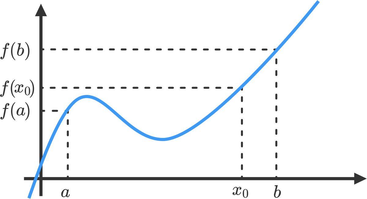 |
| The Intermediate Value Theorem states if you have a continuous function, and define (a,f(a)) and (b,f(b)), there must be at least one argument between a and b for all function values between f(a) and (b). Source: https://brilliant.org/wiki/intermediate-value-theorem/ |
 |
| The mean value theorem is also conditional on having continuous function. After taking the slope between the points (a,f(a)) and (b,f(b)), you will know that there must be at least one point on the curve where the slope is equal to this "secant" slope. Source: Robert Ortiz (https://commons.wikimedia.org/wiki/File:Mvt2.svg) |
This discussion of slopes as mentioned in the definition of the Mean Value Theorem will begin to matter very much in the lesson on Derivatives.
Answers:
First Practice (Matching Functions to Graphs): A - 5, B - 1, C - 4, D - 6, E - 3, F - 2
Second Practice (Limit based on Table): The limit is approx. .511 or .512.
Credits:
Graphs were made with Desmos and the Symbolab Graphing Calculator.
Body image affects outcomes. Self-acceptance and medical weight loss fort myers appreciation of your body’s capabilities encourages healthier habits. Avoiding negative self-talk supports a positive mental space for consistent efforts.
ReplyDeleteThis article provides a clear and insightful explanation of complex concepts. The best ebook writing company UK could take inspiration from such well-structured educational content.
ReplyDeleteUnderstanding limits in calculus, much like building a strong nursing care plan, is about mastering foundational concepts. When academic demands compete for time, seeking nursing care plan writing help from specialists allows students to ensure academic rigour while dedicating focus to complex mathematical principles and clinical proficiency.
ReplyDelete